/* -------------------------------------------------------------------
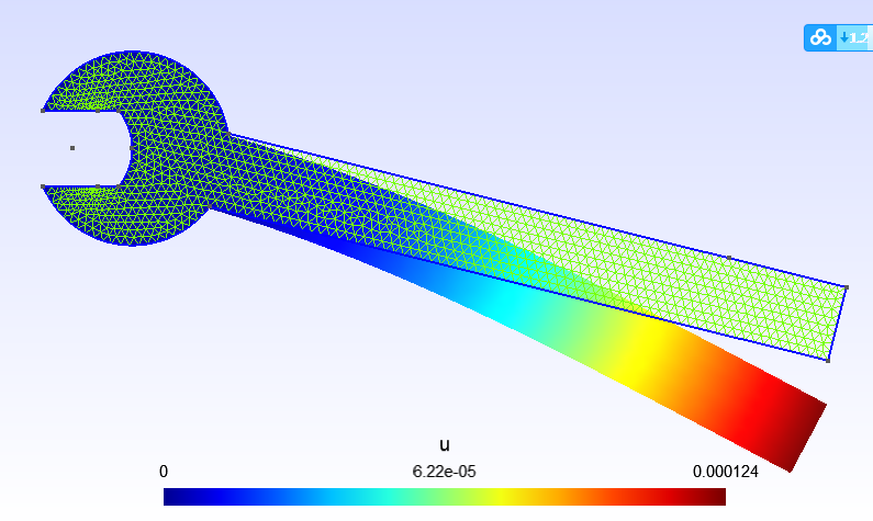
Tutorial 3 : linear elastic model of a wrench
Features:
- "grad u" GetDP specific formulation for linear elasticity
- first and second order elements
- triangular and quadrangular elements
To compute the solution in a terminal:
getdp wrench2D.pro -solve Elast_u -pos pos
To compute the solution interactively from the Gmsh GUI:
File > Open > wrench.pro
Run (button at the bottom of the left panel)
------------------------------------------------------------------- */
/*
Particularities of linear elasticity in GetDP:
Instead of a vector field "u = Vector[ ux, uy, uz ]", the displacement field
is regarded as two (2D case) or three (3D case) scalar fields.
Unlike conventional formulations, GetDP formulation is then written in terms
of the gradient "grad u" of the displacement field, which is a non-symmetric
tensor, and the needed symmetrization (to define the strain tensor and relate
it to the stress tensor) is done via the constitutive relationship (Hooke law).
This unusual formulation allows to take advantage of the powerful geometrical
and homological GetDP kernel, which relies on the operators grad, curl and div.
The "grad u" formulation entails a small increase of assembly work but makes
in counterpart lots of geometrical features implemented in GetDP (change of
coordinates, function spaces, etc...) applicable to elastic problems
out-of-the-box, since the scalar fields { ux, uy, uz } have exactly the same
geometrical properties as, e.g. an electric scalar potential or a temperature
field.
*/
Include "wrench2D_common.pro";
Young = 1e9 * DefineNumber[ 200, Name "Material/Young modulus [GPa]"];
Poisson = DefineNumber[ 0.3, Name "Material/Poisson coefficient []"];
AppliedForce = DefineNumber[ 100, Name "Material/Applied force [N]"];
// Approximation of the maximum deflection by an analytical model:
// Deflection = PL^3/(3EI) with I = Width^3*Thickness/12
Deflection = DefineNumber[4*AppliedForce*((LLength-0.018)/Width)^3/(Young*Thickness)*1e3,
Name "Solution/Deflection (analytical) [mm]", ReadOnly 1];
Group {
// Physical regions: Give explicit labels to the regions defined in the .geo file
Wrench = Region[ 1 ];
Grip = Region[ 2 ];
Force = Region[ 3 ];
// Abstract regions:
Vol_Mec = Region[ Wrench ];
Vol_Force_Mec = Region[ Wrench ];
Sur_Clamp_Mec = Region[ Grip ];
Sur_Force_Mec = Region[ Force ];
/* Meaning of abstract regions:
- Vol_Mec : Elastic domain
- Vol_Force_Mec : Region with imposed volume force
- Sur_Force_Mec : Surface with imposed surface traction
- Sur_Clamp_Mec : Surface with imposed zero displacements (all components) */
}
Function {
/*
Material coefficients
No need of regionwise definition ( E[{Wrench}] = ... ; )
as this model comprises only one region.
If there is more than one region and coefficients are not particularised,
the same value holds for all of them.
*/
E[] = Young;
nu[] = Poisson;
/*
Volume force components applied to the region "Vol_Force_Mec"
Gravity could be defined here as well ( force_y[] = 7000*9.81; ) ;
*/
force_x[] = 0;
force_y[] = 0;
/* Surface traction force components applied to the region "Sur_Force_Mec" */
pressure_x[] = 0;
pressure_y[] = -AppliedForce/(SurfaceArea[]*Thickness); // downward vertical force
}
/* Hooke's law
The material law
sigma_ij = C_ijkl epsilon_ij
is represented in 2D by four 2x2 tensors C_ij[], i,j=1,2, depending on the Lamé
coefficients of the isotropic linear material,
lambda = E[]*nu[]/(1.+nu[])/(1.-2.*nu[])
mu = E[]/2./(1.+nu[])
as follows
EPC: a[] = E/(1-nu^2) b[] = mu c[] = E nu/(1-nu^2)
EPD: a[] = lambda + 2 mu b[] = mu c[] = lambda
3D: a[] = lambda + 2 mu b[] = mu c[] = lambda
respectively for the 2D plane strain (EPD), 2D plane stress (EPS) and 3D cases.
*/
Function {
Flag_EPC = 1;
If(Flag_EPC) // Plane stress
a[] = E[]/(1.-nu[]^2);
c[] = E[]*nu[]/(1.-nu[]^2);
Else // Plane strain or 3D
a[] = E[]*(1.-nu[])/(1.+nu[])/(1.-2.*nu[]);
c[] = E[]*nu[]/(1.+nu[])/(1.-2.*nu[]);
EndIf
b[] = E[]/2./(1.+nu[]);
C_xx[] = Tensor[ a[],0 ,0 , 0 ,b[],0 , 0 ,0 ,b[] ];
C_xy[] = Tensor[ 0 ,c[],0 , b[],0 ,0 , 0 ,0 ,0 ];
C_yx[] = Tensor[ 0 ,b[],0 , c[],0 ,0 , 0 ,0 ,0 ];
C_yy[] = Tensor[ b[],0 ,0 , 0 ,a[],0 , 0 ,0 ,b[] ];
}
/* Clamping boundary condition */
Constraint {
{ Name Displacement_x;
Case {
{ Region Sur_Clamp_Mec ; Type Assign ; Value 0; }
}
}
{ Name Displacement_y;
Case {
{ Region Sur_Clamp_Mec ; Type Assign ; Value 0; }
}
}
}
/* As mentioned above, the displacement field is discretized as two scalar
fields "ux" and "uy", which are the spatial components of the vector field
"u" in a fixed Cartesian coordinate system.
Boundary conditions like
ux = ... ;
uy = ... ;
translate naturally into Dirichlet constraints on the scalar "ux" and "uy"
FunctionSpaces. More exotic conditions like
u . n = ux Cos [th] + uy Sin [th] = ... ;
are less naturally accounted for within the "grad u" formulation; but they
could be easily implemented with e.g. a Lagrange multiplier.
The finite element shape (e.g. triangles or quadrangles in 2D) has no influence
in the definition of the FunctionSpaces. The appropriate shape functions
are determined by GetDP at a much lower level on basis of the information
contained in the *.msh file.
Second order elements are hierarchically implemented by adding to the first
order node-based shape functions a set of second order edge-based functions
to complete a basis for 2D order polynomials on the reference element.
*/
// Domain of definition of the "ux" and "uy" FunctionSpaces
Group {
Dom_H_u_Mec = Region[ { Vol_Mec, Sur_Force_Mec, Sur_Clamp_Mec} ];
}
Flag_Degree = DefineNumber[ 0, Name "Geometry/Use degree 2 (hierarch.)",
Choices{0,1}, Visible 1];
FE_Order = ( Flag_Degree == 0 ) ? 1 : 2; // Convert flag value into polynomial degree
FunctionSpace {
{ Name H_ux_Mec ; Type Form0 ;
BasisFunction {
{ Name sxn ; NameOfCoef uxn ; Function BF_Node ;
Support Dom_H_u_Mec ; Entity NodesOf[ All ] ; }
If ( FE_Order == 2 )
{ Name sxn2 ; NameOfCoef uxn2 ; Function BF_Node_2E ;
Support Dom_H_u_Mec; Entity EdgesOf[ All ] ; }
EndIf
}
Constraint {
{ NameOfCoef uxn ;
EntityType NodesOf ; NameOfConstraint Displacement_x ; }
If ( FE_Order == 2 )
{ NameOfCoef uxn2 ;
EntityType EdgesOf ; NameOfConstraint Displacement_x ; }
EndIf
}
}
{ Name H_uy_Mec ; Type Form0 ;
BasisFunction {
{ Name syn ; NameOfCoef uyn ; Function BF_Node ;
Support Dom_H_u_Mec ; Entity NodesOf[ All ] ; }
If ( FE_Order == 2 )
{ Name syn2 ; NameOfCoef uyn2 ; Function BF_Node_2E ;
Support Dom_H_u_Mec; Entity EdgesOf[ All ] ; }
EndIf
}
Constraint {
{ NameOfCoef uyn ;
EntityType NodesOf ; NameOfConstraint Displacement_y ; }
If ( FE_Order == 2 )
{ NameOfCoef uyn2 ;
EntityType EdgesOf ; NameOfConstraint Displacement_y ; }
EndIf
}
}
}
Jacobian {
{ Name Vol;
Case {
{ Region All; Jacobian Vol; }
}
}
{ Name Sur;
Case {
{ Region All; Jacobian Sur; }
}
}
}
/* Adapting the number of Gauss points to the polynomial degree of the finite elements
is simple: */
Integration {
{ Name Gauss_v;
Case {
If (FE_Order == 1)
{ Type Gauss;
Case {
{ GeoElement Line ; NumberOfPoints 3; }
{ GeoElement Triangle ; NumberOfPoints 3; }
{ GeoElement Quadrangle ; NumberOfPoints 4; }
}
}
Else
{ Type Gauss;
Case {
{ GeoElement Line ; NumberOfPoints 5; }
{ GeoElement Triangle ; NumberOfPoints 7; }
{ GeoElement Quadrangle ; NumberOfPoints 7; }
}
}
EndIf
}
}
}
Formulation {
{ Name Elast_u ; Type FemEquation ;
Quantity {
{ Name ux ; Type Local ; NameOfSpace H_ux_Mec ; }
{ Name uy ; Type Local ; NameOfSpace H_uy_Mec ; }
}
Equation {
Integral { [ -C_xx[] * Dof{d ux}, {d ux} ] ;
In Vol_Mec ; Jacobian Vol ; Integration Gauss_v ; }
Integral { [ -C_xy[] * Dof{d uy}, {d ux} ] ;
In Vol_Mec ; Jacobian Vol ; Integration Gauss_v ; }
Integral { [ -C_yx[] * Dof{d ux}, {d uy} ] ;
In Vol_Mec ; Jacobian Vol ; Integration Gauss_v ; }
Integral { [ -C_yy[] * Dof{d uy}, {d uy} ] ;
In Vol_Mec ; Jacobian Vol ; Integration Gauss_v ; }
Integral { [ force_x[] , {ux} ];
In Vol_Force_Mec ; Jacobian Vol ; Integration Gauss_v ; }
Integral { [ force_y[] , {uy} ];
In Vol_Force_Mec ; Jacobian Vol ; Integration Gauss_v ; }
Integral { [ pressure_x[] , {ux} ];
In Sur_Force_Mec ; Jacobian Sur ; Integration Gauss_v ; }
Integral { [ pressure_y[] , {uy} ];
In Sur_Force_Mec ; Jacobian Sur ; Integration Gauss_v ; }
}
}
}
Resolution {
{ Name Elast_u ;
System {
{ Name Sys_Mec ; NameOfFormulation Elast_u; }
}
Operation {
InitSolution [Sys_Mec];
Generate[Sys_Mec];
Solve[Sys_Mec];
SaveSolution[Sys_Mec] ;
}
}
}
PostProcessing {
{ Name Elast_u ; NameOfFormulation Elast_u ;
PostQuantity {
{ Name u ; Value {
Term { [ Vector[ {ux}, {uy}, 0 ]]; In Vol_Mec ; Jacobian Vol ; }
}
}
{ Name uy ; Value {
Term { [ 1e3*{uy} ]; In Vol_Mec ; Jacobian Vol ; }
}
}
{ Name sig_xx ; Value {
Term { [ CompX[ C_xx[]*{d ux} + C_xy[]*{d uy} ] ];
In Vol_Mec ; Jacobian Vol ; }
}
}
{ Name sig_xy ; Value {
Term { [ CompY[ C_xx[]*{d ux} + C_xy[]*{d uy} ] ];
In Vol_Mec ; Jacobian Vol ; }
}
}
{ Name sig_yy ; Value {
Term { [ CompY [ C_yx[]*{d ux} + C_yy[]*{d uy} ] ];
In Vol_Mec ; Jacobian Vol ; }
}
}
}
}
}
PostOperation {
{ Name pos; NameOfPostProcessing Elast_u;
Operation {
If(FE_Order == 1)
Print[ sig_xx, OnElementsOf Wrench, File "sigxx.pos" ];
Print[ u, OnElementsOf Wrench, File "u.pos" ];
Else
Print[ sig_xx, OnElementsOf Wrench, File "sigxx2.pos" ];
Print[ u, OnElementsOf Wrench, File "u2.pos" ];
EndIf
Echo[ StrCat["l=PostProcessing.NbViews-1; ",
"View[l].VectorType = 5; ",
"View[l].ExternalView = l; ",
"View[l].DisplacementFactor = 200; ",
"View[l-1].IntervalsType = 3; "
],
File "tmp.geo", LastTimeStepOnly] ;
//Print[ sig_yy, OnElementsOf Wrench, File "sigyy.pos" ];
//Print[ sig_xy, OnElementsOf Wrench, File "sigxy.pos" ];
Print[ uy, OnPoint{probe_x, probe_y, 0},
File > "deflection.pos", Format TimeTable,
SendToServer "Solution/Deflection (computed) [mm]", Color "AliceBlue" ];
}
}
}
// Tell Gmsh which GetDP commands to execute when running the model.
DefineConstant[
R_ = {"Elast_u", Name "GetDP/1ResolutionChoices", Visible 0},
P_ = {"pos", Name "GetDP/2PostOperationChoices", Visible 0},
C_ = {"-solve -pos -v2", Name "GetDP/9ComputeCommand", Visible 0}
];