在OpenMX当中,可以将晶胞的多条近似重叠的能带打开成原胞仿真结果。构建大一些的晶胞可以方便我们对体系进行赝原子轨道分解,还可以仿真缺陷和掺杂的情况。
先上一个石墨烯的原胞版的能带打开范例。在这个范例当中,由于使用的是原胞,所以仿真结果和晶胞一致,即使不设置参考晶格矢量。
文件名为Graphen_C_Primitive.dat
#
# File Name
#

System.CurrrentDirectory         ./
System.Name                     graphene_c_primitive
level.of.stdout                   1    # default=1 (1-3)
level.of.fileout                  1    # default=1 (1-3)

#
# Definition of Atomic Species
#

Species.Number       1
<Definition.of.Atomic.Species
  C    C6.0-s2p2d1    C_PBE13
Definition.of.Atomic.Species>


#
# Atoms
#

Atoms.Number 2
Atoms.SpeciesAndCoordinates.Unit  Ang  # Ang|AU
<Atoms.SpeciesAndCoordinates
 1  C  0.000000000  0.710000000  0.000000000  2.0 2.0
 2  C  0.000000000  -0.71000000  0.000000000  2.0 2.0
Atoms.SpeciesAndCoordinates>

Atoms.UnitVectors.Unit             Ang   # Ang|AU
<Atoms.UnitVectors
1.22980000000000 2.13000000000000  0.00000000000000
1.22980000000000 -2.13000000000000  0.00000000000000
0.00000000000000 0.00000000000000 20.00000000000000
Atoms.UnitVectors>

#
# SCF or Electronic System
#

scf.XcType                GGA-PBE      # LDA|LSDA-CA|LSDA-PW|GGA-PBE
scf.SpinPolarization       off          # On|Off
scf.SpinOrbit.Coupling      off
scf.ElectronicTemperature  300.0       # default=300 (K)
scf.energycutoff          200.0        # default=150 (Ry)
scf.maxIter                300         # default=40
scf.EigenvalueSolver      Band         # Recursion|Cluster|Band
scf.Kgrid                10 10  1        # means n1 x n2 x n3
scf.Mixing.Type            rmm-diisk   # Simple|Rmm-Diis|Gr-Pulay
scf.Init.Mixing.Weight     0.07        # default=0.30
scf.Min.Mixing.Weight      0.003       # default=0.001
scf.Max.Mixing.Weight      0.15        # default=0.40
scf.Mixing.History         39          # default=5
scf.Mixing.StartPulay      10          # default=6
scf.Mixing.EveryPulay       1
scf.criterion             1.0e-7       # default=1.0e-6 (Hartree)

#
# MD or Geometry Optimization
#

MD.Type                   Nomd        # Nomd|Opt|DIIS|NVE|NVT_VS|NVT_NH

#
# Band dispersion
#

Band.dispersion              on       # on|off, default=off

#
# Unfolding of bands
#
Band.Nkpath                   3
<Band.kpath
   25  0.5 0.0 0.0       0.333 0.333 0.0   M  K
   25  0.333 0.333 0.0     0.0 0.0 0.0        K  G
   25  0.0 0.0 0.0       0.5 0.0 0.0        G  M
Band.kpath>

Unfolding.Electronic.Band      on     # on|off, default=off
Unfolding.LowerBound        -15.0     # default=-10 eV
Unfolding.UpperBound          15.0     # default= 10 eV

Unfolding.desired_totalnkpt    30
Unfolding.Nkpoint               4

<Unfolding.kpoint
M 0.5 0.0 0.0
K 0.333 0.333 0.0
G 0.0 0.0 0.0
M 0.5 0.0 0.0
Unfolding.kpoint>
仿真结果文件有unfold_orbup,这里面第一列是k点,第二列是对应的能量,可以用gnuplot来画1:2出(打开版的)能带。可以验证这样算出的能带和普通方式算出的能带是一样的。
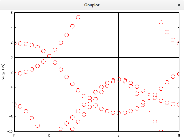
接着说上面代码的结果,上面的代码是最简单的石墨烯的能带打开仿真。出现的文件中有一个.unfold_plotexample文件。文件名为Graphene_C_Primitive_Te.dat,部分内容如下:
set yrange [-15.000000:15.000000]
set ylabel 'Energy (eV)'
set xtics('M' 0.000000,'K' 0.450166,'G' 1.350474,'M' 2.130950)
set xrange [0:2.130950]
set arrow nohead from 0,0 to 2.130950,0
set arrow nohead from 0.450166,-15.000000 to 0.450166,15.000000
set arrow nohead from 1.350474,-15.000000 to 1.350474,15.000000
set style circle radius 0
plot 'graphene_c_primitive.unfold_totup' using 1:2:($3)*0.05 notitle with circles lc rgb 'red'
只要仿真没错,都会有这个文件。
可以用gnuplot 的load命令直接load这个文件

就可以画出图
貌似为了仿真倒带性质,OpenMX用户手册在SiC的例子里添加了一个Te空原子。我们也在石墨烯的仿真文件中照猫画虎,添加一个Te空原子,修改后的部分文件内容和仿真结果如下:
Species.Number       2
<Definition.of.Atomic.Species
  C    C6.0-s2p2d1    C_PBE13
  Te  Te11.0-s2p2d2f1  E
Definition.of.Atomic.Species>


#
# Atoms
#

Atoms.Number 3
Atoms.SpeciesAndCoordinates.Unit  Ang  # Ang|AU
<Atoms.SpeciesAndCoordinates
 1  C  0.000000000  0.710000000  0.000000000  2.0 2.0
 2  C  0.000000000  -0.71000000  0.000000000  2.0 2.0
 3  Te 1.229800000   0.00000000  0.000000000  0   0
Atoms.SpeciesAndCoordinates>

Atoms.UnitVectors.Unit             Ang   # Ang|AU
<Atoms.UnitVectors
1.22980000000000 2.13000000000000  0.00000000000000
1.22980000000000 -2.13000000000000  0.00000000000000
0.00000000000000 0.00000000000000 20.00000000000000
Atoms.UnitVectors>
将晶胞扩充为原胞
我们继续将晶胞扩充为原胞,诸多细节不再列举。代码如下:
#
# File Name
#
System.CurrrentDirectory ./
System.Name graphene_c_nsp_p
level.of.stdout 1 # default=1 (1-3)
level.of.fileout 1 # default=1 (1-3)
#
# Definition of Atomic Species
#
Species.Number 1
<Definition.of.Atomic.Species
C C7.0-s2p2d1 C_PBE13
Definition.of.Atomic.Species>
#
# Atoms
#
Atoms.Number 8
Atoms.SpeciesAndCoordinates.Unit Ang # Ang|AU
<Atoms.SpeciesAndCoordinates
1 C 0.000000000 0.710000000 0.000000000 2.0 2.0
2 C 0.000000000 -0.71000000 0.000000000 2.0 2.0
3 C 1.2298 2.8400 0.00000 2.0 2.0
4 C 1.2298 1.4200 0.00000000 2.0 2.0
5 C 1.2298 -1.4200 0.00000000 2.0 2.0
6 C 1.2298 -2.8400 0.000000000 2.0 2.0
7 C 2.4596 0.7100 0.00000000 2.0 2.0
8 C 2.4596 -0.7100 0.000000000 2.0 2.0
Atoms.SpeciesAndCoordinates>
Atoms.UnitVectors.Unit Ang # Ang|AU
<Atoms.UnitVectors
2.45960000000000 4.26000000000000 0
2.45960000000000 -4.26000000000000 0
0 0 40
Atoms.UnitVectors>
#
# SCF or Electronic System
#
scf.XcType GGA-PBE # LDA|LSDA-CA|LSDA-PW|GGA-PBE
scf.SpinPolarization off # On|Off
scf.ElectronicTemperature 300.0 # default=300 (K)
scf.energycutoff 200.0 # default=150 (Ry)
scf.maxIter 300 # default=40
scf.EigenvalueSolver Band # Recursion|Cluster|Band
scf.Kgrid 5 5 1 # means n1 x n2 x n3
scf.Mixing.Type rmm-diisk # Simple|Rmm-Diis|Gr-Pulay
scf.Init.Mixing.Weight 0.07 # default=0.30
scf.Min.Mixing.Weight 0.003 # default=0.001
scf.Max.Mixing.Weight 0.15 # default=0.40
scf.Mixing.History 39 # default=5
scf.Mixing.StartPulay 10 # default=6
scf.Mixing.EveryPulay 1
scf.criterion 1.0e-7 # default=1.0e-6 (Hartree)
#
# MD or Geometry Optimization
#
MD.Type Nomd # Nomd|Opt|DIIS|NVE|NVT_VS|NVT_NH
#
# Band dispersion
#
Band.dispersion on # on|off, default=off
Band.Nkpath 3
<Band.kpath
25 0.5 0.0 0.0 0.333 0.333 0.0 M K
25 0.333 0.333 0.0 0.0 0.0 0.0 K G
25 0.0 0.0 0.0 0.5 0.0 0.0 G M
Band.kpath>
#
# Unfolding of bands
#
Unfolding.Electronic.Band on # on|off, default=off
Unfolding.LowerBound -10.0 # default=-10 eV
Unfolding.UpperBound 6.0 # default= 10 eV
Unfolding.desired_totalnkpt 30
Unfolding.Nkpoint 4
<Unfolding.kpoint
M 0.5 0.0 0.0
K 0.333 0.333 0.0
G 0.0 0.0 0.0
M 0.5 0.0 0.0
Unfolding.kpoint>
<Unfolding.ReferenceVectors
1.22980000000000 2.13000000000000 0.00000000000000
1.22980000000000 -2.13000000000000 0.00000000000000
0.00000000000000 0.00000000000000 20.00000000000000
Unfolding.ReferenceVectors>
<Unfolding.Map
1 1
2 2
3 1
4 2
5 1
6 2
7 1
8 2
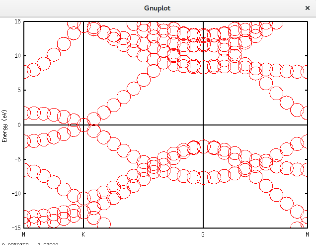
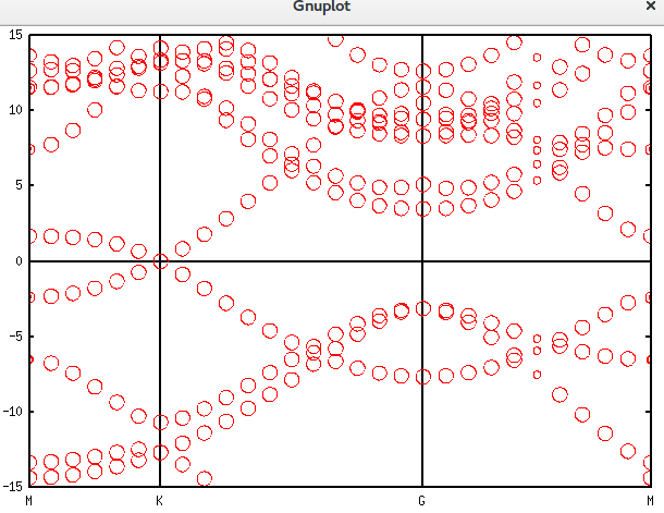
Unfolding.Map>用上面介绍的gnuplot方法画出结果:
带隙还在,可以接受。再进一步,填入空隙,结果如下。可以发现,圆圈多了很多。代码放在附录里面。Graphene_C_NSP_P_Te.dat
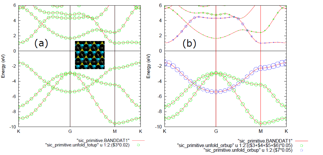
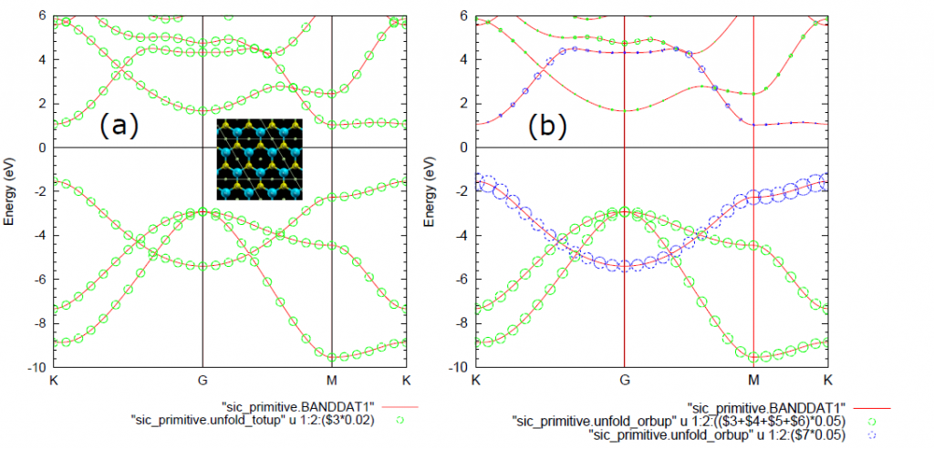
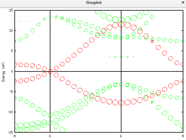
上面的是总的totup文件的数据。要获得赝原子轨道分解的数据需要将unfold_plotexample文件的代码写成如下这样:
set yrange [-15.000000:15.000000]
set ylabel 'Energy (eV)'
set xtics('M' 0.000000,'K' 0.450166,'G' 1.350474,'M' 2.130950)
set xrange [0:2.130950]
set arrow nohead from 0,0 to 2.130950,0
set arrow nohead from 0.450166,-15.000000 to 0.450166,15.000000
set arrow nohead from 1.350474,-15.000000 to 1.350474,15.000000
set style circle radius 0
plot 'graphene_c_nsp_p_te.unfold_orbup' using 1:2:(($3+$4+$5+$6)*0.5) notitle with circles lc rgb 'green','graphene_c_nsp_p_te.unfold_orbup' using 1:2:($7*0.5) notitle with circles lc rgb 'red'
得到的图形如下:
仿真掺杂
在石墨烯表面掺入一个磷原子,能带的移动可以用上面的理论与方法直观地看到了。对应的仿真文件为名为Graphene_C_NSP_V.dat。该文件也放在附录当中。
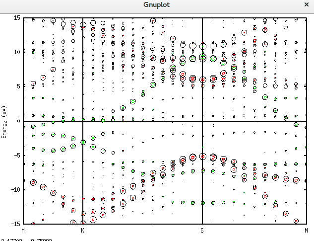
而画出它这个图的plotexample文件为:
set yrange [-15.000000:15.000000]
set ylabel 'Energy (eV)'
set xtics('M' 0.000000,'K' 0.450166,'G' 1.350474,'M' 2.130950)
set xrange [0:2.130950]
set arrow nohead from 0,0 to 2.130950,0
set arrow nohead from 0.450166,-15.000000 to 0.450166,15.000000
set arrow nohead from 1.350474,-15.000000 to 1.350474,15.000000
set style circle radius 0
plot 'graphene_c_nsp_v.unfold_orbup' using 1:2:($4+$5+$6)*0.2 notitle with circles lc rgb 'red','graphene_c_nsp_v.unfold_orbup' using 1:2:($7)*0.2 notitle with circles lc rgb 'green','graphene_c_nsp_v.unfold_totup' using 1:2:($3)*0.05 notitle with circles lc rgb 'black'
使用Band.kpath和Band.Nkpath命令来控制产生能带数据。如果不要能带,这个就可以不写。产生的.Band文件要用gnuband13处理。
Band.Nkpath 3
<Band.kpath
25 0.5 0.0 0.0 0.333 0.333 0.0 M K
25 0.333 0.333 0.0 0.0 0.0 0.0 K G
25 0.0 0.0 0.0 0.5 0.0 0.0 G M
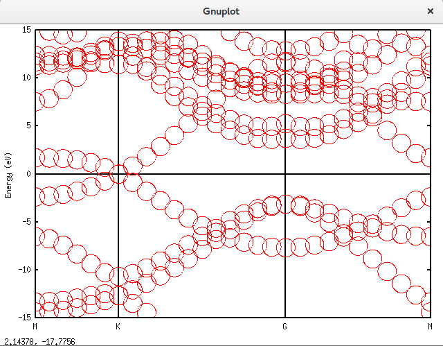
Band.kpath>处理之后,把BANDDAT1的数据和unfold_orbup文件画在一个图中
plot "graphene_c_nsp_v.BANDDAT1" using ($1*2):2 w l lc rgb 'green','graphene_c_nsp_v.unfold_orbup' using 1:2:($4+$5+$6)*0.2 notitle with circles lc rgb 'red','graphene_c_nsp_v.unfold_orbup' using 1:2:($7)*0.2 notitle with circles lc rgb 'blue'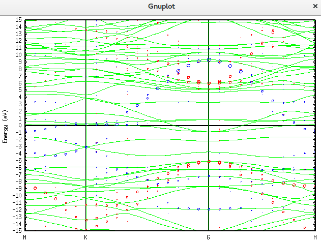
附注
Graphene_C_NSP_P_Te.dat
#
# File Name
#

System.CurrrentDirectory         ./
System.Name                     graphene_c_nsp_p_te
level.of.stdout                   1    # default=1 (1-3)
level.of.fileout                  1    # default=1 (1-3)

#
# Definition of Atomic Species
#

Species.Number       2
<Definition.of.Atomic.Species
  C    C7.0-s2p2d1    C_PBE13
  Te Te11.0-s2p2d2f1  E
Definition.of.Atomic.Species>


#
# Atoms
#

Atoms.Number 12
Atoms.SpeciesAndCoordinates.Unit  Ang  # Ang|AU
<Atoms.SpeciesAndCoordinates
 1  C  0.000000000  0.710000000  0.000000000  2.0 2.0
 2  C  0.000000000  -0.71000000  0.000000000  2.0 2.0
 3  Te 1.2298000000   0.00000000  0.000000000   0   0
 4  C  1.2298        2.8400      0.00000      2.0 2.0
 5  C  1.2298       1.4200       0.00000000   2.0 2.0
 6  Te  2.4596       2.1300       0.0          0   0
 7  C  1.2298       -1.4200      0.00000000    2.0 2.0
 8  C  1.2298       -2.8400      0.000000000  2.0 2.0
 9  Te  2.4596       -2.1300         0         0   0
 10  C  2.4596      0.7100       0.00000000   2.0 2.0
 11  C  2.4596      -0.7100      0.000000000  2.0 2.0
 12  Te 3.6894         0         0              0   0
Atoms.SpeciesAndCoordinates>

Atoms.UnitVectors.Unit             Ang   # Ang|AU
<Atoms.UnitVectors
2.45960000000000	4.26000000000000	0
2.45960000000000	-4.26000000000000	0
0	                 0	               40
Atoms.UnitVectors>

#
# SCF or Electronic System
#

scf.XcType                GGA-PBE      # LDA|LSDA-CA|LSDA-PW|GGA-PBE
scf.SpinPolarization       off          # On|Off
scf.ElectronicTemperature  300.0       # default=300 (K)
scf.energycutoff          200.0        # default=150 (Ry)
scf.maxIter                300         # default=40
scf.EigenvalueSolver      Band         # Recursion|Cluster|Band
scf.Kgrid                10 10  1        # means n1 x n2 x n3
scf.Mixing.Type            rmm-diisk   # Simple|Rmm-Diis|Gr-Pulay
scf.Init.Mixing.Weight     0.07        # default=0.30
scf.Min.Mixing.Weight      0.003       # default=0.001
scf.Max.Mixing.Weight      0.15        # default=0.40
scf.Mixing.History         39          # default=5
scf.Mixing.StartPulay      10          # default=6
scf.Mixing.EveryPulay       1
scf.criterion             1.0e-7       # default=1.0e-6 (Hartree)

#
# MD or Geometry Optimization
#

MD.Type                   Nomd        # Nomd|Opt|DIIS|NVE|NVT_VS|NVT_NH

#
# Band dispersion
#

Band.dispersion              on       # on|off, default=off

Band.Nkpath                   3
<Band.kpath
   25  0.5 0.0 0.0       0.333 0.333 0.0   M  K
   25  0.333 0.333 0.0     0.0 0.0 0.0        K  G
   25  0.0 0.0 0.0       0.5 0.0 0.0        G  M
Band.kpath>

#
# Unfolding of bands
#

Unfolding.Electronic.Band      on     # on|off, default=off
Unfolding.LowerBound        -15.0     # default=-10 eV
Unfolding.UpperBound         15.0     # default= 10 eV

Unfolding.desired_totalnkpt    30
Unfolding.Nkpoint               4

<Unfolding.kpoint
M 0.5 0.0 0.0
K 0.333 0.333 0.0
G 0.0 0.0 0.0
M 0.5 0.0 0.0
Unfolding.kpoint>

<Unfolding.ReferenceVectors
1.22980000000000 2.13000000000000  0.00000000000000
1.22980000000000 -2.13000000000000  0.00000000000000
0.00000000000000 0.00000000000000 20.00000000000000
Unfolding.ReferenceVectors>


<Unfolding.Map
  1 1
  2 2
  3 3
  4 1
  5 2
  6 3
  7 1
  8 2
  9 3
  10 1
  11 2
  12 3
Unfolding.Map>
Graphene_C_NSP_V.dat
#
# File Name
#

System.CurrrentDirectory         ./
System.Name                     graphene_c_nsp_v
level.of.stdout                   1    # default=1 (1-3)
level.of.fileout                  1    # default=1 (1-3)

#
# Definition of Atomic Species
#

Species.Number       2
<Definition.of.Atomic.Species
  C    C7.0-s2p2d1    C_PBE13
 P      P8.0-s2p2d1   P_CA13
Definition.of.Atomic.Species>


#
# Atoms
#

Atoms.Number 9
Atoms.SpeciesAndCoordinates.Unit  Ang  # Ang|AU
<Atoms.SpeciesAndCoordinates
 1  C  0.000000000  0.710000000  0.000000000  2.0 2.0
 2  C  0.000000000  -0.71000000  0.000000000  2.0 2.0
 3  C  1.2298        2.8400      0.00000      2.0 2.0
 4  C  1.2298       1.4200       0.00000000   2.0 2.0
 5  C  1.2298       -1.4200      0.00000000    2.0 2.0
 6  C  1.2298       -2.8400      0.000000000  2.0 2.0
 7  C  2.4596      0.7100       0.00000000   2.0 2.0
 8  C  2.4596      -0.7100      0.000000000  2.0 2.0
 9  P  1.229800000  0.00000000  1.520000000  2.5 2.5
Atoms.SpeciesAndCoordinates>

Atoms.UnitVectors.Unit             Ang   # Ang|AU
<Atoms.UnitVectors
2.45960000000000	4.26000000000000	0
2.45960000000000	-4.26000000000000	0
0	                 0	               40
Atoms.UnitVectors>

#
# SCF or Electronic System
#

scf.XcType                GGA-PBE      # LDA|LSDA-CA|LSDA-PW|GGA-PBE
scf.SpinPolarization       off          # On|Off
scf.ElectronicTemperature  300.0       # default=300 (K)
scf.energycutoff          200.0        # default=150 (Ry)
scf.maxIter                300         # default=40
scf.EigenvalueSolver      Band         # Recursion|Cluster|Band
scf.Kgrid                5 5  1        # means n1 x n2 x n3
scf.Mixing.Type            rmm-diisk   # Simple|Rmm-Diis|Gr-Pulay
scf.Init.Mixing.Weight     0.07        # default=0.30
scf.Min.Mixing.Weight      0.003       # default=0.001
scf.Max.Mixing.Weight      0.15        # default=0.40
scf.Mixing.History         39          # default=5
scf.Mixing.StartPulay      10          # default=6
scf.Mixing.EveryPulay       1
scf.criterion             1.0e-7       # default=1.0e-6 (Hartree)

#
# MD or Geometry Optimization
#

MD.Type                   Nomd        # Nomd|Opt|DIIS|NVE|NVT_VS|NVT_NH

#
# Band dispersion
#

Band.dispersion              on      # on|off, default=off
Band.Nkpath                3
<Band.kpath
   25  0.5 0.0 0.0       0.333 0.333 0.0   M  K
   25  0.333 0.333 0.0     0.0 0.0 0.0        K  G
   25  0.0 0.0 0.0       0.5 0.0 0.0        G  M
Band.kpath>

#
# Unfolding of bands
#

Unfolding.Electronic.Band      on     # on|off, default=off
Unfolding.LowerBound        -15.0     # default=-10 eV
Unfolding.UpperBound         15.0     # default= 10 eV

Unfolding.desired_totalnkpt    30
Unfolding.Nkpoint               4

<Unfolding.kpoint
M 0.5 0.0 0.0
K 0.333 0.333 0.0
G 0.0 0.0 0.0
M 0.5 0.0 0.0
Unfolding.kpoint>

<Unfolding.ReferenceVectors
1.22980000000000 2.13000000000000  0.00000000000000
1.22980000000000 -2.13000000000000  0.00000000000000
0.00000000000000 0.00000000000000 20.00000000000000
Unfolding.ReferenceVectors>


<Unfolding.Map
  1 1
  2 2
  3 1
  4 2
  5 1
  6 2
  7 1
  8 2
  9 3
Unfolding.Map>